This is a webified version
of the paper
in The
Mathematica Journal, vol. 7 no. 3, 1999.
My original Mathematica notebook
for just the code is here,
but Russell
Towle has since expanded upon this code
and has an updated notebook
available.
Zonohedrification
George W. Hart
Abstract
An efficient algorithm is presented to construct arbitrary zonohedra
and to "zonohedrify" a given polyhedron. There are relatively few interesting
processes which input an arbitrary polyhedron and output a related polyhedron.
Well-known examples are truncation, stellation, dualization (reciprocation
in a sphere), and compounding. To this list, can be added zonohedrification,
in which the vertex directions of the original polyhedron (relative to
an arbitrary center) determine the edge directions of the resulting zonohedrification.
A few mathematical properties of zonohedra are outlined, to give the reader
insight into zonohedral structure and an understanding of the algorithm.
Background
Zonohedra are beautiful, interesting polyhedra bounded by zonogons,
where a zonogon is a polygon in which the edges come in equal opposite
parallel pairs. The faces and the solid are necessarily centrally symmetric,
and may have additional symmetries. In the special case where all the faces
happen to be four-sided, a zonohedron is bounded by parallelograms.
Some simple, zonohedra are shown in Figure 1. All are easily generated
by the algorithm presented below. In addition to their aesthetic quality,
zonohedra are the form of certain mineral crystals, they are projections
into 3-space of higher dimensional hypercubes, they pop up in the analysis
of quasi-regular "Penrose" tilings of the plane, they have been proposed
as architectural structures, and a number of familiar polyhedra happen
to be zonohedra. One special type of zonohedron is the polar zonohedron,
which was illustrated in the Spring, 1996 issue of this Journal [1]. Three
excellent references [2, 3, 4] discuss the general case at the recreational,
undergraduate, and graduate levels respectively. From a mathematical perspective,
zonohedra are particularly notable for the way in which they intertwine
combinatorial and geometric properties. One relevant theorem [3, p. 28]
is that if each face of a convex polyhedron is centrally symmetric, then
the entire solid is centrally symmetric. We only consider convex zonohedra
here; two interesting nonconvex zonohedra are illustrated in [3, p. 103].
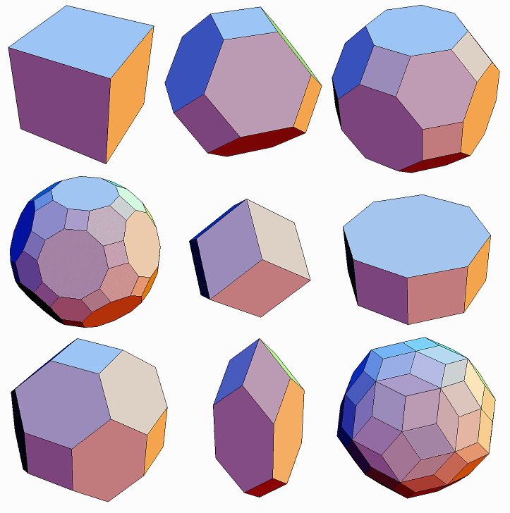
|
| Figure 1. Some familiar polyhedra which are zonohedra: (a)
cube, (b) truncated octahedron, (c) truncated cuboctahedron, (d) truncated
icosidodecahedron, (e) rhombic dodecahedron, (f) octagonal prism, (g) truncated
rhombic dodecahedron, (h) elongated dodecahedron, (i) rhombic enneacontahedron.
These have respectively 3, 6, 9, 15, 4, 5, 7, 5, and 10 zones, and are
the zonohedrifications of an octahedron, cuboctahedron, tetrakis cube (i.e.,
replace each face of a cube with a low square pyramid), icosidodecahedron,
cube, octagonal pyramid, square pyramid, and dodecahedron. |
The zonohedra illustrated in Figure 1 are zonohedrifications of other
polyhedra listed in the caption. The geometric relation between a polyhedron,
P,
and its zononedrification, Z, is the following: For every plane
defined by the center, v0, of P and (at least)
two vertices, v1, v2, of P
there
are two equal opposite faces of Z parallel to that plane. Furthermore,
these two opposite faces of Z have edges which are parallel to and
equal to the lines v0v1 and
v0v2.
Furthermore, every edge of Z comes about in that manner, i.e., every
edge is congruent and parallel to a line v0vi
for some vertex vi of P.
As an example, given an octahedron, we can find three different planes
each defined by two vertices and the octahedron's center. (Each plane happens
to contain 4 vertices.) Evidently, the six faces of a (properly oriented
and scaled) cube come in pairs parallel to these three orthogonal planes,
and the edges of the cube are each equal and parallel to some line connecting
a vertex of the octahedron with its center. We write cube=Z[octahedron],
where
Z[P]
indicates
the zonohedrification of P. (Coincidentally, the cube is also the
dual
of
the octahedron; usually the dual and the zonohedrification are distinct.)
To continue the example, we find that Z[cube], i.e., Z[Z[octahedron]],
is
the rhombic dodecahedron. Observe in Figure 1e that the edges of the rhombic
dodecahedron are each in one of four directions, corresponding to the four
diagonals of the cube. Continuing, Z[Z[Z[octahedron]]],
i.e., Z[rhombic
dodecahedron], is a form of truncated rhombic dodecahedron (Figure
1g). The process can be nested indefinitely, producing a sequence of new
polyhedra starting with any polyhedron.
The definition above assumes that v0 (the center of
P)
is well defined. If P has a center of symmetry, it is a natural
choice for v0, but the zonohedrification of an arbitrary
irregular polyhedron will depend on what point we choose to call v0.
The software below takes the origin as v0. Starting with
a square pyramid (half an octahedron), the zonohedrification is still a
cube if v0 is chosen to be the center of the base, but
an elongated dodecahedron (Figure 1h) if v0 lies above
or below the center of the base. The elongated dodecahedron is notable
for being one of the five convex solids which are space-filling by translation
(without rotation or reflection). These five solids, Figures 1a, b, e,
h, and 3b, are each the Voronoi cell of a three-dimensional lattice and
so any sheared or stretched version is equally space filling. They were
first enumerated by the Russian crystallographer E. S. Fedorov, who originally
defined and studied zonohedra a century ago.
To appreciate zonohedra, one must see their zones. Given one
edge of any zonohedron, there exists a set of equal parallel edges, e.g.,
four vertical edges of a cube. A zone is the set of faces which contain
edges from that set, e.g. four vertical faces of the cube. Such a set must
form a band which encircles the zonohedron like a belt. This is because,
by definition, all the faces are zonogons, so given an edge, a face incident
with that edge has an equal opposite edge, and one can hop from edge to
edge moving across a face with each hop and stepping only on equal parallel
edges. As there are only a finite number of such edges, eventually the
sequence of hops must return to the starting edge.
From this circumhopping construction, it follows that a zonohedron has
a number of zones equal to the number of different edge directions and,
in fact, the set of edge directions determines the zonohedron. If we consider
each edge direction vector to be rooted at the origin, we have what is
called a star of n vectors. When we zonohedrify a polyhedron,
we will use its vertices to determine the star and then the star will determine
the generated polyhedron. If the vectors in the star are of equal length,
the edges of the resulting zonohedron are equal, and it is called an equilateral
zonohedron. For example, Figure 1h is not equilateral; by shortening
its vertical edges an equilateral zonohedron can be obtained. Similarly,
any zonohedron can be made equilateral, i.e., unit length vectors can be
chosen for the star.
If a zonohedron is made entirely of parallelograms and has more than
three zones, one can remove any zone from it and assemble the two disconnected
pieces to obtain a smaller zonohedron, with one less zone. Figure 2 illustrates
this process starting with (a) the 6-zone 30-face rhombic triacontahedron.
(It is Z[icosahedron]; the twelve vertices of an icosahedron lie
on six "long diagonal" lines which define the zonal edge directions.) By
steps, it is first reduced to (b) a 5-zone 20-face rhombic icosahedron
(which is a polar zonohedron, Z[pentagonal antiprism]), then (c)
the 4-zone 12-face rhombic dodecahedron of the second kind [Footnote
1], and finally (d) a 3-zone 6-face parallelepiped.
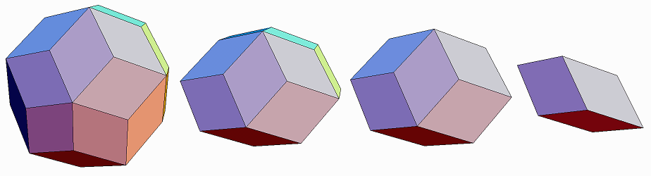
|
| Figure 2. By a series of zone removals, any zonohedron bounded
by parallelograms is reducible to a parallelepiped. In each step, a zone
is removed and the two remaining "hemispheres" are brought together. Starting
with (a) the rhombic triacontahedron, we get (b) a rhombic icosahedron,
(c) a rhombic dodecahedron of the second kind, and (d) a parallelepiped.
The reverse process can be used in a zonohedra construction algorithm. |
Observe in the previous paragraph that n-zone zonohedra have
n(n-1)
faces.
This is always the case when a zonohedron is bounded by parallelograms.
The reason is easily seen if one observes that every pair of zones intersects
twice, at two opposite faces. As there are (n
choose 2) =
n(n-1)/2
possible
pairs of zones, it follows that there are n(n-1)
faces. In the general
case, where some zonogon faces have more than 4 sides, there will be fewer
faces, as some faces are the intersection of 3 or more zones. The combinatorics
of counting faces, edges, and vertices is interesting, but not needed here.
One can reverse the zone-removal process of Figure 2 and write an algorithm
which constructs a zonohedron zone-by-zone, but I have found that approach
to be relatively slow. Before describing a faster method, let me first
mention and dismiss an even slower method.
If an n-dimensional hypercube is linearly projected into 3-space,
the convex hull of the projection is an n-zone zonohedron. Figure
3 shows how a 4-dimensional hypercube projects into 3-space giving a 4-zone
solid which can be either (a) a skewed version of the rhombic dodecahedron
or (b) a hexagonal prism. Hexagonal faces arise if three of the hypercube's
edge directions are projected into coplanar vectors. A relatively simple
program can carry out these steps, but is prohibitively slow because the
hypercube has 2n vertices. Although the final zonohedron
(after taking the convex hull) has a number of components which is polynomial
in n, the intermediate steps require time which is exponential in
n.
So the method is unsuitable for the larger examples below, but it leads
to a useful data structure for zonohedral components.
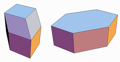
|
| Figure 3. Projecting a 4-dimensional hypercube into 3-space
and looking at its exterior typically gives (a) an object whose exterior
is a skewed rhombic dodecahedron. In the special case where the projections
of three hypercube edges happen to be coplanar, the result can be (b) an
irregular hexagonal prism. |
Data Structures
Effective data structures, appropriate to the problem domain, are essential.
To begin with, the star is simply a list of n 3-vectors, each given
by an {x, y, z} coordinate representation. The order of the vectors in
the star is not important as it will be treated like a set. For the examples
of Figure 3, I chose:
starFig3a={{1,0,0}, {0,1,0},
{0,0,1}, {-1/2, 1/2, 1/2}}
starFig3b={{1,0,0}, {0,1,0},
{0,0,1}, {1,1,0}}
In the first case, four vectors in general position were selected, i.e.,
no three vectors are coplanar, so the result is bounded by parallelograms.
In the second case, three vectors lie in a plane, and so the zonohedron
contains hexagons in parallel planes.
We next define a "p-representation" to represent parts
such as faces, edges, and vertices. Observe that there are three possible
positions for a part relative to the nth zone: the part can be entirely
on one side of the nth zone, entirely on the other side of the zone,
or (if not a vertex) it can span the zone. We represent any part with a
list of n elements in which the nth component is respectively
1, -1, or 0. Figure 4 illustrates this representation with the examples
of Figure 3. The sign of any +/-1 is understood in terms of the corresponding
element of the star. Observe that a hexagon representation has three zeros
as it spans three zones, a parallelogram has two zeros, an edge has 1 zero,
and a vertex representation has zero zeros, i.e., it consists entirely
of 1's and -1's. These are just the Cartesian coordinates in n-space
of the center of the edge-two hypercube component which is the preimage
of the part.
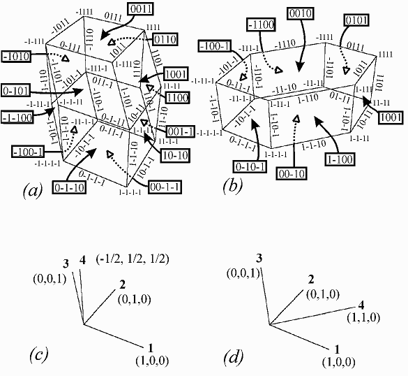
|
| Figure 4. The parts of an n-zone zonohedron are named with
an n-vector of 0's, 1's, and -1's. The star for (a) is (c); the star for
(b) is (d). Both have four zones, but in (b,d), three zonal directions
are coplanar giving a hexagonal face. |
One useful property of this representation is that a part p is
centrally opposite the part -p. For another, notice that a part
p1
is a subpart of p2 iff p2 is 0 in all
positions where they differ. So, to find the two endpoints of an edge,
we replace the 0 in its representation first with 1 and then with -1. There
is also a simple method to find the edge opposite a given edge, p1,
within a given face, p2. We simple negate those components
of p1 which are zero in p2, while keeping
the other components unchanged, i.e., compute 2 p2 -
p1.
Finally, we need a data structure for a complete polyhedron which can
be the input and output of a zonohedrify
function, so we can nest it. The format we will use is that a polyhedron
is a list of faces, a face is a list of vertices (in a cyclic order around
the perimeter), and a vertex is an {x, y, z} triple. Mathematica provides
a package of polyhedra, but in a different form. The built-in function
Vertices
returns a list of a built-in polyhedron's vertices, in {x, y, z} form.
The built-in function Faces
provides a list of its faces, where each face is represented as a list
of indices into Vertices.
We define a function builtInPolyto
convert a built-in polyhedron from that format into our format.
builtInPoly[polyhedron_]
:=
Map[Vertices[polyhedron][[#]]&,
Faces[polyhedron], {2}]
We can easily extract the vertices of a polyhedron in our format:
vertices[poly_] := Union[Flatten[poly,
1]]
The following function takes a polyhedron in our format and displays
it with Mathematica's 3D graphics. Each face must be headed with
Polygon.
view[poly_] := Show[Graphics3D[Map[Polygon,
poly]],
Boxed->False]
For example, to load the polyhedra package and then convert and display
the built-in icosahedron, we type:
<<Graphics`Polyhedra`
view[builtInPoly[Icosahedron]]
Procedures
With the above background and data structures, we will now build up
the zonohedrification procedures in a bottom-up manner. First, a standard
3-space cross product produces a 3-vector orthogonal to two given vectors.
cross[ {ax_, ay_, az_},
{bx_, by_, bz_} ] :=
{ay bz - az by, az bx - ax bz, ax by - ay bx}
Closely related is the next procedure, which tests if two vectors are
collinear. Ideally, collinear vectors have a cross product of {0, 0, 0},
but I have included a small leeway of 0.000001 in the zero test here, because
the Graphics`Polyhedra` database
gives floating point values. (This should be modified to an exact test
of zero if one starts with exact vertex coordinates.)
tolerance = 0.000001
collinear[ v1_, v2_ ]
:=
Apply[And,
Map[Abs[#]<tolerance&, cross[v1,v2]]]
We will build the star by choosing vertices one by one from the set
of vertices of the given polyhedron. Only nonzero vertices not collinear
with any vertices already selected are chosen. The following routine makes
this selection then prints out the number of zonal directions. It is convenient
to use a global variable gStar
in many of the routines below because the star remains constant in a single
zonohedrification. The last line of this routine sets this global variable,
so it need not be continuously passed from one routine to the next. (The
elements of gStar
are halved because the distance from +1 to -1 in p-representations
is 2.)
setStar[vlist_] :=
Module[{selected={}},
Scan[Function[v, If[v!={0,0,0} &&
Select[selected, collinear[v,#]&]=={},
AppendTo[selected,v]] ], vlist];
Print[Length[selected]," zonal directions."];
gStar=selected/2] (* set global variable *)
The number of zonal directions is often half the number of vertices
of the original polyhedron because in centrally symmetric polyhedra (unlike
the tetrahedron for example) vertices come in diametrically opposed pairs,
and one from each pair suffices. For example, although a cube has eight
vertices, it is centrally symmetric, so there are only four noncollinear
directions, and Z[cube] = Z[tetrahedron]. Thus, setStar[vertices[builtInPoly[Cube]]];
prints
out 4 zonal directions.
We will need a function for converting a vertex from our p representation
to {x,y,z} coordinates, i.e., projecting from n-space, treating
the star as a transformation matrix. Given a vertex p, this adds
or subtracts the vectors in the star, according to whether the components
of p are +1 or -1.
pToXYZ[p_] := Apply[Plus,
MapThread[Times, {gStar,p}]]
We also need a function to compute a vector normal to the plane of a
face. Because a face spans at least two zones, (more if it has more than
4 sides) its p contains at least two zeros. We find the zeros with
Position
and use subscripting to unpack the first two indexes. The cross product
of the corresponding elements in the star gives the normal vector.
faceNormal[p_] := With[{
indices = Position[p,0] },
cross[gStar[[indices[[1,1]]]],
gStar[[indices[[2,1]]]] ]]
The next function determines the two endpoints of a given edge. We assume
the argument has a single 0 and replace it once with -1 and once with +1:
endPoints[p_] :=
{Map[If[#==0,-1,#]&,
p], Map[If[#==0,1,#]&, p]}
Because each of a zonohedron's faces are defined by two (or more) of
the n vectors in its star, we will find it useful to have a function
which creates a list of all pairs {i, j} where 1<=i<j<=n.
For example, allPairs[4] returns{{1,2},
{1,3}, {1,4}, {2,3}, {2,4}, {3,4}}.
allPairs[n_] := With[{
indices=Table[i, {i,n}] },
Select[Flatten[Outer[List,indices,indices],1],
#[[1]]<#[[2]]&]]
To make a face parallel to the ith and jth star vector,
the convexity of the zonohedron is implicitly used. The following routine
first determines a normal vector to a plane containing those edge directions.
Then it checks the vectors of the star to see on which side of this plane
they point. That is accomplished by examining the dot product of the normal
with each vector of the star. The dot product of a vector and the normal
to the plane is zero for vectors in the plane, positive for vectors pointing
across the plane one way, and negative for vectors pointing across the
plane the other way. At least two must be zero (because the ith
and jth lie in the plane), but others may also be if the zonohedron
contains larger zonogons. Again a tolerance is used in the zero test, because
we can not expect exact planarity from floating point vertex coordinates.
makeFace[{i_,j_}] :=
With[{ normal=cross[gStar[[i]],
gStar[[j]]] },
Map[approxSign[normal.#]&, gStar]]
approxSign[x_] := If[Abs[x]<tolerance,
0, Sign[x]]
Applying makeFace to
all of the pairs {i,j} with i<j produces a list of half
the faces. The other half, i.e., the {j,i}, are geometrically opposite,
so we save a little time by generating them as -p for every p
in the first half. The following function allFaces
thereby generates a list of the p representations of all the faces.
The Union operation
is required to eliminate duplicate entries which result when a face is
generated by three (or more) coplanar entries, e.g., {i,j}, {i,k}, and
{j,k}.
allFaces :=
With[{halfTheFaces=Map[makeFace,
allPairs[Length[gStar]]]},
Union[halfTheFaces, -halfTheFaces]]
Given this list of all faces, we need to find the edges which bound
each. The procedures are analogous, because a zonogon face is a 2-dimensional
zonotope. (A zonotope is an arbitrary-dimension generalization of
the 3D zonohedron.) Three differences are (1) that normal directions for
each edge are chosen to lie in the plane of the face, (2) we don't test
every component of the star, just the ones which lie in the face, and (3)
after finding half the edges, the other half are chosen to lie geometrically
opposite not across the entire solid, but opposite within the face, using
the 2 p2 - p1 formula discussed
above. The first function below takes an argument i which is the
index of one of the zeros in p, and returns the edge of the face
that has a zero at that position. The second function applies this to all
the edge directions of a given face.
makeEdge[i_, p_, faceNormal_]
:=
With[{normal=cross[gStar[[i]],
faceNormal]},
MapThread[If[#1!=0,
#1, approxSign[#2.normal]]&,
{p, gStar}]]
makeEdges[p_] :=
With[{normal=faceNormal[p]},
With[{halfEdges=Map[makeEdge[#, p, normal]&,
Flatten[Position[p, 0]]]},
Union[halfEdges, Map[2p-#&, halfEdges]]]]
With the above routines, we have the components required to generate
a line drawing of the edges of any zonohedron. The following first finds
the edges for each face, and flattens them into a list of all edges. Then
each edge in p form is converted to a Line
with two endpoints in {x,y,z} format.
allEdges := Union[Flatten[Map[makeEdges,
allFaces], 1]]
lineDrawing :=
Map[Line[Map[pToXYZ,
endPoints[#]]]&, allEdges]
Show[Graphics3D[lineDrawing],
Boxed->False]
Line drawing graphic output is illustrated in Figure 4. However, to
generate our polyhedron format and solid graphics3D output, we need a further
step to create a polygon for each face, consisting of its vertices sorted
into a correct cyclic order. The following function does this by creating
a list of edges and vertices which are parts of a given face. It applies
the cycleSort routine
described below to the vertices.
makePolygon[p_] :=
With[{edges=makeEdges[p]},
With[{vertices=Union[Flatten[Map[endPoints,
edges],1]]},
cycleSort[Map[pToXYZ, vertices]]]]
The cyclesort routine
arranges the vertices in a cyclic order by using a two-argument arctangent
function to compute an angle for each vertex as seen from the centroid.
A general-purpose sortBy
function sorts any list according to a given numeric function of its elements.
The sorting Function[{x,y}, N[x[[1]]]<N[y[[1]]]]
explicitly converts the arctangents to numerical form to avoid the problem
of Mathematicas built-in Sort
function putting 0 before both p and -p
.
cycleSort[vertices_] :=
With[{centroid=Apply[Plus,vertices]/Length[vertices]},
sortBy[ArcTan[(#-centroid).(vertices[[1]]-centroid),
(#-centroid).(vertices[[2]]-centroid)]&, vertices]]
sortBy[fn_, list_] :=
Map[#[[2]]&,
Sort[Map[{fn[#],#}&, list,
Function[{x,y}, N[x[[1]]]<N[y[[1]]]]]]
Putting everything together, the following takes a polyhedron, makes
a star from its vertices, and outputs the zonohedrification.
zonohedrify[poly_] :=
setStar[vertices[poly]];
Map[makePolygon,
allFaces]
Examples
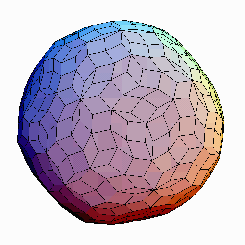
To generate the rhombic triacontahedron (Figure 2a) and then its zonohedrification
(Figure 5), we can type:
rhombicTriacontahedron
=
zonohedrify[builtInPoly[Icosahedron]];
view[rhombicTriacontahedron];
view[zonohedrify[rhombicTriacontahedron]]
|
|
Figure 5. The zonohedrification of the rhombic triacontahedron.
|
Using Nest, we
can construct, Z[Z[Z[octahedron]]], the truncated rhombic dodecahedron
of Figure 1g, . The result is composed of squares and hexagons, and is
easy to confuse with the truncated octahedron (Figure 1b) if one doesn't
look carefully.
view[Nest[zonohedrify,
builtInPoly[Octahedron], 3]]
The zonohedrify
procedure can also create a zonohedron from any arbitrary star if we embed
the star in a list (so it appears like the vertices of one face of a polyhedron).
For example, to generate the hexagonal prism of Figure 3b using the star
defined above:
view[zonohedrify[ {starFig3b}
]]
A polar zonohedron, illustrated in [1], is the zonohedrification of
a prism or antiprism. Although prisms and antiprisms are not present in
the built-in polyhedra package, their zonohedrifications can be created
with a star of vectors arranged like the ribs of an umbrella:
polarStar[n_] :=
Table[{Sin[2
Pi i/n], Cos[2 Pi i/n], 1}, {i,1,n}]//N;
view[zonohedrify[ {polarStar[10]}
]]
Particularly interesting zonohedra result if we use the symmetry axes
of a regular polyhedron as the star. These axes pass through the vertices,
face centers, and edge midpoints of a regular polyhedron, so the following
three auxiliary routines are useful.
faceCenters[poly_] :=
Map[Apply[Plus,
#]/Length[#]&, poly]
edgeMidpoints[poly_] :=
Union[Flatten[Map[(#+RotateLeft[#])/2&,
poly],1]]
unit[v_] := v/Sqrt[v.v]
With them, we can create a list of the 31 axes of symmetry of an icosahedron
(six 5-fold axes through the vertices, ten 3-fold axes through the face
centers, and fifteen 2-fold axes through the edge midpoints) to use as
a star. The function unit
provides a unit-length vector in the given direction, so the result is
an equilateral zonohedron.
view[zonohedrify[{Map[unit,
Join[
vertices[builtInPoly[Icosahedron]],
faceCenters[builtInPoly[Icosahedron]],
edgeMidpoints[builtInPoly[Icosahedron]]
]]}]]
The resulting 31-zone, 242-face polyhedron is shown as Figure 6. It
has been proposed [6] as the basis for an architectural system, akin to
geodesic domes but with a smaller inventory of parts and a greater variety
of forms.
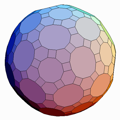
|
|
Figure 6. 31-zone zonohedron based on the 31 axes of
symmetry of the icosahedron (242 faces).
|
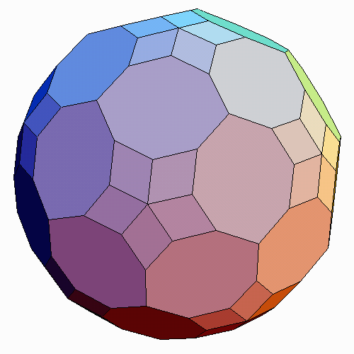
One final example is the zonohedrification of the truncated cuboctahedron.
This is the largest of fifteen paper zonohedra models shown in Plate II
of [3]. It is easy to generate if we first create a truncated cuboctahedron
(Figure 1c) as the zonohedrification of a star of the three 4-fold axes
and six 2-fold axes of a cube.
truncatedCuboctahedron
= zonohedrify[{Map[unit,
Join[faceCenters[builtInPoly[Cube]],
edgeMidpoints[builtInPoly[Cube]] ]]}];
view[zonohedrify[truncatedCuboctahedron]]
The result, shown here as Figure 7, has 24 zones and 552 parallelogram
faces.
|
|
Figure 7. The zonohedrification of the truncated cuboctahedron
(24-zones, 552 faces).
|
Conclusions
An intricate but fast algorithm has been presented which creates the
zonohedrification of a polyhedron or an arbitrary star of vectors. It can
be used to generate and display a wide variety of interesting, new polyhedra
of which a few are shown here. The electronic supplement contains a notebook
which generates all these examples.
The only output format illustrated here is Graphics3D,
but conversion to other formats is straightforward. Three-dimensional virtual
reality versions of these zonohedra are available for viewing on the internet
at [7]. A different approach to zonohedra is given in [8], which appeared
after this was written.
Notes
-
The usual rhombic dodecahedron (Figure 1e) and the rhombic dodecahedron
of the second kind (Fig 2c) each have twelve identical rhombic faces, but
of different shapes. Johannes Keppler discovered the first, but the
origin of the second is unclear. Although Coxeter [3, p. 31] cites
a 1960 reference as its first publication, I have observed that it appears
in the form of a pop-up paper model (!) in a 1752 geometry text [5].
References
-
Russell Towle, "Polar Zonohedra," Mathematica Journal, Vol. 6, No.
2, Spring, 1996, pp. 8-12.
-
W.W. Rouse Ball and H.S.M. Coxeter, Mathematical Recreations and Essays,
New York, 1938; 11th ed., (Dover reprint, 1960).
-
H.S.M. Coxeter, Regular Polytopes, Macmillan, 1963, (Dover reprint,
1973).
-
Gunter M. Ziegler, Lectures on Polytopes, Springer-Verlag, 1995.
-
John Lodge Cowley, Geometry Made Easy, 1752.
-
Steve Baer, Zome Primer, Zomeworks, P.O. Box 712, Albuquerque, New
Mexico.
-
http://www.li.net/~george/virtual-polyhedra/vp.html
-
David Eppstein, "Zonohedra and Zonotopes," Mathematica in Education
and Research, Vol. 5, No. 4, pp. 15-21, 1996.